Swap Rates from Implied forward and Spot Rates

I will give an overview of the swap rates and how this is constructed from the implied forward and spot rates.

First, we need Depo’s and EuroDollar futures which are liquid and exchange traded instruments from which the $O/N, T/N, S/N, 1M, 3M, 6M, 9M, 12M$ rates can be formed. Eurodollar instruments yields the futures rates and applying this with the convexity, we can then derive the implied forward rates.

Now to the next section, we need to price swap, lets say 1Y2Y swap. First, we need to get the 2 year swap rate for which we need to value both legs to zero. The answer is the “average” of the first two years of the forward curve, specifically the sequence of forward rates on 3-month LIBOR.

In general market makers set the bid and ask rates on over-the-counter (OTC) derivatives such as forwards and swaps based on the cost and risk of the most efficient way of hedging risk. When available, actively traded futures contract offer the best hedge. Note that main difference between forward and futures is settling arrangement. Whereas forward are settled as per contract agreement on the expiry dates, futures are daily settled and margins accrued typically every day.

$forward_t = futures_t - \frac{1}{2} \sigma T_1 T_2$

Why is the forward interest rate lower than the otherwise comparable futures rate? The key is that the gains and losses on an OTC forward contract are realized in a lump sum at the delivery date.

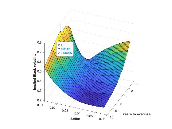
Stochastic Modelling of Volatility

There are many stochastic volatility modelling approaches that fit each use cases for instance, DD (displacement diffusion) is used modelling inflation, CEV (constant elasticity of variance) used modelling FX, interest rates, LMM, SABR etc., There isn’t one model that fits all. Therefore trader needs to make judgement based on the market forecast and implied prices how he/she perceives the future and uses the appropriate model to quote the price and hedge the risk. Note that pricing is easy, as one can always take the market quoted prices and calibrate given model to replicate the plain vanilla prices. But most important aspect of any good modelling theory is how well it implies the future hedging cost, as therefore predicts if not accurately but approximately the future slope of the underlying asset movement.

We will discuss one such model, proposed in early 2002 by Hagan et all, SABR, called Stochastic Alpha Beta and Rho model. This model is proposed to alleviate the dynamics of local volatility model which was proposed by Dupire, Derman and Kani which while calibrates today’s plain vanilla option prices perfectly but wrongly predicts the dynamics of future smile.

The original SABR model shifts the underlying, hence the delta risk changes which is improved by Bernlett’s new improved SABR model. We will see below how to include the new modified delta and vega risk.

SABR ATM vol, $sigma_{ATM}$ is given by,

$\sigma_{ATM} = \frac{\alpha_0}{f^{1-\beta}}\{ 1 + [\frac{(1-\beta)^2}{24}\frac{\alpha_0^2}{f^{2-2\beta}} + \frac{\rho \beta \nu \alpha_0}{4 f^{1-\beta}} + \frac {2 -3\rho^2}{24} \nu^2] T \}$

Stochastic Alpha Beta Rho – Volatility Smiles

Resources

https://www.mathworks.com/help/fininst/pricing-a-swaption-using-the-sabr-model.html

Click to access Gatheral.1.pdf

Click to access v_sibetz_nowak.pdf

Click to access MatlabMasterScript.pdf

Ito’s Partial Differential Equation

We will derive the Ito’s PDE for lognormal process and derive the solution.

Suppose given process A_t follows geometric brownian motion under \textbf{P} pricing measure,
$dA_t = \mu A_t dt + \sigma A_t dW_t$
The same process under \textbf{Q} pricing measure given by,
$dA_t = r A_t dt + \sigma A_t dW_t$

Now, let’s suppose we have process,

$dX_t = a(X_t, t) dt + b(X_t, t) dW_t$
Let’s suppose, we have Y_t = g(X_t, t)
By Ito’s process, we know that,
$dY_t = \frac{dg}{dt} + \frac{dg}{dX} X_t + \frac{1}{2} \frac{d^2g}{dX^2} (dX_t)^2$

Now, we from brownian motion properties, $dt^2 = 0, dW dt = 0, dW^2 = dt$ . Applying them,

$dY_t = \frac{dg}{dt} + \frac{dg}{dt}(a(X_t, t)dt + b(X_t, t) dW_t) + \frac{1}{2} \frac{d^2g}{dt^2} (b^2 (X_t, t)dt)$

Now, since we know $Y = ln A_t$ , therefore, $\frac{dg}{dx} = \frac{1}{X}, \frac{d^2g}{dX^2} = \frac{-1}{X^2}$ . We now apply,

$dY_t = \frac {1}{A} dA + \frac{1}{2} {-1}{A^2} (dA)^2$
$dY_t = \mu dt + \sigma dW_t - \frac{1}{2} \sigma^2 dt$
$dY_t = (\mu - \frac{1}{2} \sigma_2) dt + \sigma dW_t$

Now, integrating now RHS,

$Y_t = Y_0 + (\mu - \frac{1}{2} \sigma^2) dt + \sigma dW_t$

We know that $Y_t = ln(A_t)$ , so applying, we get the final derivation,

$A_t = A_0 + exp ( (\mu + \frac{1}{2} \sigma^2) dt + \sigma dW_t )$

Structural Credit Merton Model

We will see how to derive the structural credit merton model, another way from reduced form model, where the default is modelled from the underlying market traded debt.

$E_T = max( A_T - D, 0)$
$E_t = A_t N(d_1) - D e-^{rT} N(d_2)$
$d1 = \frac {ln (\frac{Ae^{rT}}{D})}{\sigma_A \sqrt{T}} + \frac{1}{2} \sigma_A \sqrt{T}$

Now, the leverage can be written as, $L = \frac{\hat{D}}{A}$ , where $\hat{D} = D_0 e^{(r - y)T}$

Now, equity call on the underlying debt can be written in terms of leverage, asset vol and time to maturity as,

$E_t = A_t [ N(d_1) + L N(d_2) ]$
$d1 = \frac {-ln(L) + (r + \frac{\sigma_A^2}{T} ) T}{\sigma_A \sqrt{T}}$

Credit Value Adjustments (CVA)

CVA’s can be priced unilaterally or bilaterally. We will see some of the terms in CVA,

Future Exposure (FE):
Underlying positive (simulated) future exposure.
$E(t_j, \omega_s) := (V(t_j, \omega_s)^{+}) = max(V(t_j, \omega_s), 0)$
Worst Potential Future Exposure (WPFE):
Maximum positive future exposure
$EE(t_j) = max(E(t_j, \omega_s))$

Let’s now focus on the steps involved in CVA pricing, note that, CVA pricing given below

$CVA = LGD (PD_{(0, T)}) D_{(0, T)} E[max(V_j,0)^+]$

1. Price the forward contract
2. Compute the max exposure on each scenario
3. Price for the CVA
4. Subtract from the forward price determined from #1 to get the overall exposure

Let’s see how to compute CVA from 2-step binomial forward price process.